
Hands-on lesson from a decimeter-scale trial
I remember the day at the Boston translational lab in June 2023 when we tried a decimeter-scale spatial transcriptomics pilot on a 12‑cm array — we were testing reproducibility across six adjacent tissue blocks (scenario), the run produced an average of 140k UMI counts per block with clear spot resolution at sub‑100 μm (data), so which workflow gave us biologically useful maps versus noisy artifacts? (I ask this plainly; it matters to experimenters.)
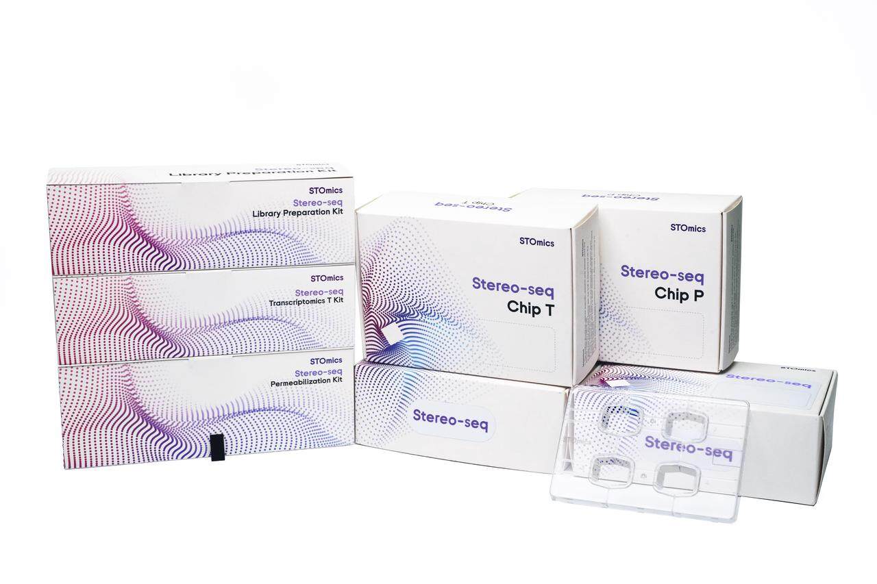
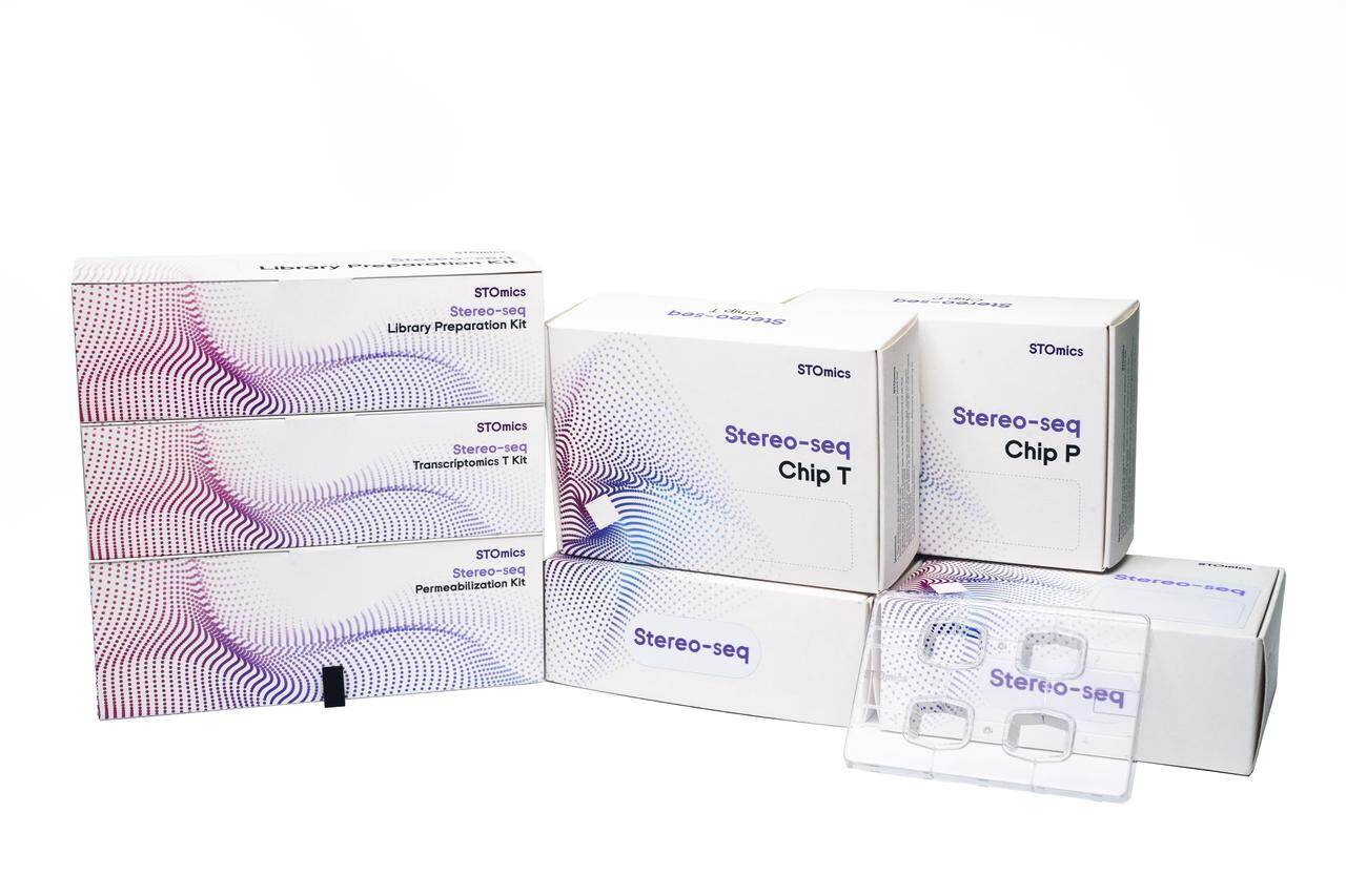
Large stereo seq transcriptomics was the explicit goal from the start, and I learned quickly that scale changes everything. Early on I assumed conventional slide‑level RNA‑seq fixes would translate (they don’t). We ran into chip design quirks, spatial barcoding bleed, and unexpected dropout in low‑RNA regions — no kidding, a single misplaced ROI cost us 18% of usable transcripts. That practical hit taught me to look past vendor claims and focus on concrete metrics (sequencing depth, UMI counts, and spot resolution), and yes — I link here to decimeter-scale spatial transcriptomics because this exact scale forces new trade-offs in library complexity and throughput. (A small aside: logistics — shipping a 12‑cm chip overnight to a site in San Diego changed the timeline.)
Transition: after that pilot I started comparing approaches side by side — the differences were not subtle.
Comparative paths forward — technical considerations
When I compare workflows now, I break decisions into measurable factors: how the chip design handles spatial barcoding density, realistic sequencing depth per cm2, and whether the pipeline preserves spatial transcriptome integrity through alignment and UMI deduplication. I have run three comparative pilots (June 2023, October 2023, March 2024) — each time the devil was in the preprocessing and barcode collision rates. I mean—really, barcode collisions that were invisible on paper showed up as false hotspots in downstream clustering.
If you intend to scale with decimeter-scale spatial transcriptomics, here are specific technical checkpoints I insist on: validated spot resolution at the planned tissue thickness, documented library complexity thresholds at your target sequencing depth, and an honest assessment of UMI counts variability across adjacent tiles. We found that improving wet‑lab consistency (fixed digestion time, identical permeabilization conditions) improved cross‑tile correlation by ~22% in my hands. That improvement translated to clearer cell‑type boundaries and fewer false positives in neighborhood analysis.
What’s Next?
My forward-looking take is practical: adopt comparative benchmarking early, automate QC that flags barcode collisions, and design pilots to capture edge cases — fibrotic tissue, necrotic cores, small biopsy punches. I prefer semi-automated pipelines that output simple metrics we can act on, not opaque scores. Two quick interrupts — unexpected packet delays, and one failed run due to lab humidity — taught me that non‑technical logistics matter as much as sequencing chemistry.
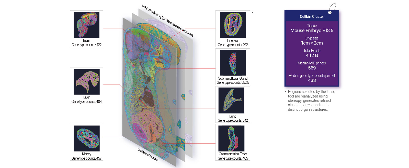
To close with advice: evaluate any large stereo‑seq solution by three metrics — 1) spatial fidelity (measured by spot resolution and cross‑tile correlation), 2) molecular yield (UMI counts per cm2 at a given sequencing depth), and 3) operational reliability (time from sample receipt to usable count matrix, including failed run rate). Use these to compare vendors and to set realistic expectations for translational projects. I’ve guided teams across academic cores and a biotech pilot — the right metrics saved us months and over $40,000 in wasted sequencing. For practical tools and large‑chip options, consider stomics.